Page 4 - Demo

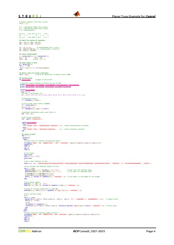
Planar Truss Example for Comrel Add-on RCP Consult, 2021-2026 Page 4%% Boundary conditions% Applied loadsfc = zeros(ndof,1);fc(16:2:26) = -P; % negative vertical forces [N] % Supports and free nodesc = [1 2 14]; % fixed dofs d = setdiff(1:ndof,c); % free dofs % Remove supports from force vectorfc(c) = []; % f = equivalent nodal force vector% q = equilibrium nodal force vector% a = displacements%| qd | | Kcc Kcd || ac | | fd |%| | = | || | - | |%| qc | | Kdc Kdd || ad | | fc |%% Solve the system of equationsKcc = K(c,c); Kcd = K(c,d);Kdc = K(d,c); Kdd = K(d,d);ac = [0; 0; 0]; % displacements for c are 0ad = Kdd\\(fc-Kdc*ac); % = linsolve(Kdd, fc-Kdc*ac)qd = Kcc*ac + Kcd*ad;%% Final displacementsa = zeros(ndof,1); q = zeros(ndof,1);a(c) = ac; q(c) = qd;a(d) = ad; % q(d) = qc = 0%% Axial loads in barsN = zeros(nfe,1);for e = 1:nfe N(e) = k(e)*[-1 0 1 0]*T{e}*a(LM{e});end%% Return value of script (function)uout = a(8); % vertical deflection at bottom center (N04)%% Visualisationif StrurelPlot % begin of plot block %% Global variables to manage plot facilities global StrurelPlotName StrurelPlotType StrurelPlotMode StrurelPlotCount StrurelPlotName='PlanarTruss_'; StrurelPlotType='.png'; StrurelPlotMode=3; % Internal values defined in Strurel to use in plot global StrurelName StrurelMode StrurelModule StrurelVersion StrurelEngine global StrurelIMET StrurelIOPT StrurelBeta StrurelPf StrurelRun switch(StrurelMode) case {0, 2} % X and Y coordinates in m XY = [0 0; 4 0; 8 0; 12 0; 16 0; 20 0; 24 0; 22 2; 18 2; 14 2; 10 2; 6 2; 2 2]; % Deflection vector b = reshape(a,[2,nnp])'; % Forces with scale factor 0.000025 fc = zeros(ndof,1); fc(16:2:26) = P; d = reshape(fc,[2,nnp])'*0.000025; % Deformed coordinates with scale factor 2. DEF = XY + b*2; % Get screen resolution pxl = get(0,'screensize'); switch(StrurelMode) case 0 tit='Planar Truss - Deterministic Solution'; % 0 - initial deterministic solution case 2 tit='Planar Truss - Stochastic Solution'; % 2 - final stochastic solution end %% Create 3 plots for f = 1:3 switch(f) case 1 % Center plot for initial and deformed states ff(1)=figure('Name', tit, 'NumberTitle', 'off', 'Position', [pxl(3)/4 pxl(4)/4 pxl(3)/2 pxl(4)/2]); figure(ff(1)) hold on box on view(2) % Plot frame axis equal axis([-2 26 -2 10]) grid minor % Set a main subtitle of plot text(12.0, 8.0, '\\fontsize{16}\\color{blue}Initial \\color{black}and \\color{red}deformed \\color{black}states', 'FontSize', 16, 'HorizontalAlignment','center'); % Plot initial and deformed states of truss for e = 1:nfe plot(XY(IEN(e,:),1), XY(IEN(e,:),2), 'b-'); % blue color for initial state plot(DEF(IEN(e,:),1), DEF(IEN(e,:),2), 'r-'); % red color for deformed state x=(XY(IEN(e,1),1)+XY(IEN(e,2),1))/2; y=(XY(IEN(e,1),2)+XY(IEN(e,2),2))/2; text(x, y, strcat('R',num2str(e')), 'FontSize', 8); % rod number in the middle of rod length end