Page 6 - Demo

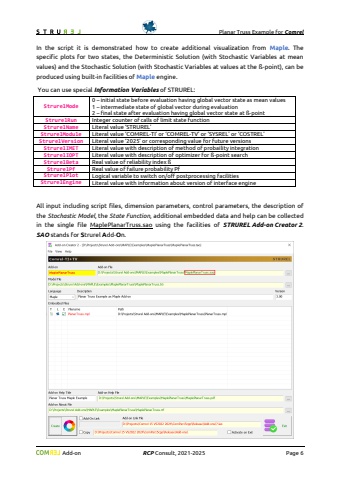
Planar Truss Example for Comrel Add-on RCP Consult, 2021-2026 Page 6 # plot set #3 PlotS:=[seq(BarS[i],i=1..nfe),seq(AS[i],i=1..nfe),seq(mapC[i],i=1..nco),seq(mapL[i],i=1..2)]: end if: # Plot frame Rplt:=rectangle([-2,-1],[28,7],transparency=1,thickness=0.5): # Plot values of input data A1p:=textplot([23.5,4.7,`#msup(mi(` || (sprintf(\ A2p:=textplot([23.5,4.4,`#msup(mi(` || (sprintf(\ E1p:=textplot([23.5,4.1,`#msup(mi(` || (sprintf(\ E2p:=textplot([23.5,3.8,`#msup(mi(` || (sprintf(\ # Plot a main title of plot if StrurelMode = 0 or StrurelMode = 2 then : T1p:=textplot([0.5,4.6,sprintf(\right},font=[\ end if: if StrurelMode = 0 then : # input data at state of mean values T2pt:=\ T3pt:=\ elif StrurelMode = 2 then : # input data at beta-point T2pt:=sprintf(\ T3pt:=sprintf(\ end if: T2p:=textplot([0.5,4.3,T2pt],align={above,right},font=[\ T3p:=textplot([0.5,4.0,`` || T3pt || ``],align={above,right},font=[\ Tse:=textplot([0,-1,StrurelEngine],align={above,right},font=[\ display(Rplt, PlotT, PlotS, A1p, A2p, E1p, E2p, T1p, T2p, T3p, Tse, scaling=constrained,axis=[thickness=0.5,gridlines=[color=lightblue]],title=tit,titlefont=[\ end proc: for np to 3 do if StrurelPlotMode = 1 or StrurelPlotMode = 3 then # Complete maplet to display a created plot mapletS := Maplet(Plotter('width'=getmetric(0)/2,'height'=getmetric(1)/2,'reference'='Plotter','value'=TrussPlot(np)), # plot function defined above BoxLayout('reference'='BoxLayout', BoxColumn(BoxCell('value'='Plotter'))), Window('layout'='BoxLayout','reference'='Window','resizable'='false','title'=tit), Action(RunWindow('window'='Window'))): # Show maplet Maplets[Display](mapletS): end if: if StrurelPlotMode = 2 or StrurelPlotMode = 3 then ++StrurelPlotCount: Export(cat(StrurelPlotName,convert(StrurelPlotCount,string),StrurelPlotType),TrussPlot(np), width=getmetric(0)/2,height=getmetric(1)/2): end if: end do: end if:end if: # end of plot block## Return value of script (proc)return a[8]; # vertical deflection at bottom center (N04)end proc:## Procedure to create \Jet := proc(n)c:=Matrix(n,3,fill=1.):dv:=2/(n-1):v:=-1;for i to n do if v < -0.5 then c[i,1]:=0.: c[i,2]:=4*(v+1.)/2.: elif v < 0. then c[i,1]:=0.: c[i,3]:=1.+4*(-0.5-v)/2: elif v < 0.5 then c[i,1]:=4*v/2: c[i,3]:=0.: else c[i,2]:=1.+4*(0.5-v)/2: c[i,3]:=0: end if: v:=v+dv:end do:return c:end:In the script it is demonstrated how to create additional visualization from Maple. The specific plots for two states, the Deterministic Solution (with Stochastic Variables at mean values) and the Stochastic Solution (with Stochastic Variables at values at the %u00df-point), can be produced using built-in facilities of Maple engine.