Page 4 - Demo

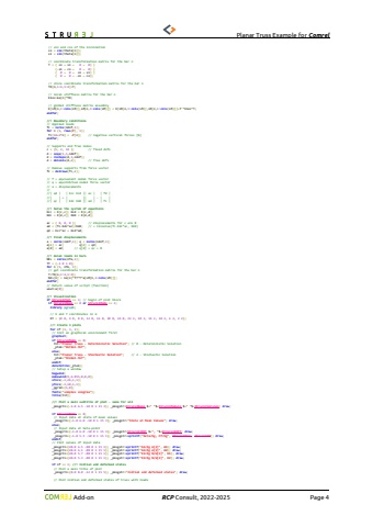
Planar Truss Example for Comrel Add-on RCP Consult, 2022-2025 Page 4 // sin and cos of the inclination co = cos(theta[n]); si = sin(theta[n]); // coordinate transformation matrix for the bar n T = ( co ~ si ~ 0 ~ 0) | (-si ~ co ~ 0 ~ 0) | ( 0 ~ 0 ~ co ~ si) | ( 0 ~ 0 ~ -si ~ co); // store coordinate transformation matrix for the bar n Tb[n,1:4,1:4]=T; // local stiffness matrix for the bar n Kloc=ke[n]*TD; // global stiffness matrix assembly K[LM[n,1:cols(LM)],LM[n,1:cols(LM)]] = K[LM[n,1:cols(LM)],LM[n,1:cols(LM)]]+T'*Kloc*T;endfor;//! Boundary conditions// Applied loadsfc = zeros(ndof,1);for n (1, rows(P), 1); fc[14+2*n] = -P[n]; // negative vertical forces [N]endfor; // Supports and free nodesc = {1, 2, 14 }; // fixed dofsd = seqa(1,1,ndof);d = reshape(d,1,ndof);d = delcols(d,c); // free dofs // Remove supports from force vectorfc = delrows(fc,c); // f = equivalent nodal force vector// q = equilibrium nodal force vector// a = displacements////| qd | | Kcc Kcd || ac | | fd |//| | = | || | - | |//| qc | | Kdc Kdd || ad | | fc |//! Solve the system of equationsKcc = K[c,c]; Kcd = K[c,d];Kdc = K[d,c]; Kdd = K[d,d];ac = { 0, 0, 0 }; // displacements for c are 0ad = (fc-Kdc*ac)/Kdd; // = linsolve(fc-Kdc*ac, Kdd)qd = Kcc*ac + Kcd*ad;//! Final displacementsa = zeros(ndof,1); q = zeros(ndof,1);a[c] = ac; q[c] = qd;a[d] = ad; // q[d] = qc = 0//! Axial loads in barsNEL = zeros(nfe,1);TT = {-1 0 1 0};for n (1, nfe, 1); // get coordinate transformation matrix for the bar n T=Tb[n,1:4,1:4]; NEL[n] = ke[n]*TT*T*a[LM[n,1:cols(LM)]];endfor;// Return value of script (function)uout=a[8];//! Visualizationif StrurelPlot == 1; // begin of plot block if StrurelMode == 0 or StrurelMode == 2; library pgraph; // X and Y coordinates in m XY = {0 0, 4 0, 8 0, 12 0, 16 0, 20 0, 24 0, 22 2, 18 2, 14 2, 10 2, 6 2, 2 2}; //! Create 3 plots for nf (1, 3, 1); // Init an graphical environment first graphset; if StrurelMode == 0; tit=\Deterministic Solution\// 0 - Deterministic Solution _ptek=\ else; tit=\Stochastic Solution\// 2 - Stochastic Solution _ptek=\ endif; deleteFile(_ptek); // Setup a window begwind; makewind(9,6.855,0,0,0); xtics(-2,26,1,1); ytics(-2,10,1,1); _pgrid={1,0}; fonts(\ title(tit); //! Plot a main subtitle of plot - same for all _pmsgctl={-1.0 6.5 .10 0 1 15 3}; _pmsgstr=StrurelName $+\$+\draw; if StrurelMode == 0; // Input data at state of mean values _pmsgctl={-1.0 6.0 .10 0 1 15 3}; _pmsgstr=\draw; else; // Input data at beta-point _pmsgctl={-1.0 6.0 .10 0 1 15 3}; _pmsgstr=StrurelIMET $+\draw; _pmsgctl={-1.0 5.5 .10 0 1 15 1}; _pmsgstr=sprintf(\StrurelBeta, StrurelPf); draw; endif; // Plot values of input data _pmsgctl={20.0 6.5 .08 0 1 15 1}; _pmsgstr=sprintf(\draw; _pmsgctl={20.0 6.1 .08 0 1 15 1}; _pmsgstr=sprintf(\draw; _pmsgctl={20.0 5.7 .08 0 1 15 1}; _pmsgstr=sprintf(\E1); draw; _pmsgctl={20.0 5.3 .08 0 1 15 1}; _pmsgstr=sprintf(\E2); draw; if nf == 1; //! Initial and deformed states // Plot a main title of plot _pmsgctl={8.0 8.0 .12 0 1 15 5}; _pmsgstr=\draw; // Plot initial and deformed states of truss with loads